Visualizing Classification Results: Confusion Star and Confusion Gear
16 Jan 2022Authors: Amalia Luque\(^1\), Mirko Mazzoleni\(^2\), Alejandro Carrasco\(^3\) and Antonio Ferramosca\(^2\)
\(^1\) Departamento de Ingeniería del Diseño, Escuela Politécnica Superior, Universidad de Sevilla, 41011 Seville, Spain
\(^2\) Department of Management, Information and Production Engineering, University of Bergamo, 24044 Dalmine, Italy
\(^3\) Departamento de Tecnología Electrónica, School of Computer Engineering, Universidad de Sevilla, 41012 Seville, Spain
In this post, we present two new visualization tools, called confusion star and confusion gear, for the representation of classification performance of multiclass classifiers. More details can be found in the paper [1]:
You can cite the paper as:
@ARTICLE{9658486,
  author={Luque, Amalia and Mazzoleni, Mirko and Carrasco, Alejandro and Ferramosca, Antonio},
  journal={IEEE Access},
  title={Visualizing Classification Results: Confusion Star and Confusion Gear},
  year={2022},
  volume={10},
  number={},
  pages={1659-1677},
  doi={10.1109/ACCESS.2021.3137630}
}
Matrices for representing classification results
We start our discussion by presenting three matrices:
-
the confusion matrix, used to represent the number of correctly and incorrectly classified instances;
-
the hits matrix, used to represent the number of correctly classified instances;
-
the errors matrix, used to represent the number of incorrectly classified instances.
Confusion matrix
Classification results from machine learning algorithms are commonly summarized in the form of a confusion matrix, especially for representing a dichotomous (\(2\)-classes) classification tasks. As the name suggests, a confusion matrix is a table representing the number of correctly and incorrectly classified instances, see Table 1.
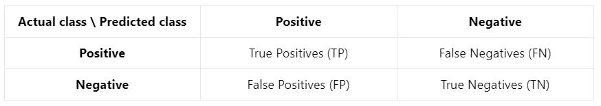 Table 1: Binary confusion matrix for a \(2\)-classes classification task
In the two-classes case, this matrix representation is visually effective: it is immediately clear if the classifier is performing well, as the number of false positives and false negatives should be as low as possible.
However, this representation suffers when more than two classes are present. A simple way to visualize the results of a \(C\)-classes classification problem (when \(C>2\)) would be to employ a one-vs-all strategy:
-
select a class to be the “Positive” one. All the other classes will constitute the “Negative” class;
-
build a binary confusion matrix representing the Positive vs. Negative classes. Repeat this process until all classes played the role of the “Positive” one;
-
visualize the \(C\) binary confusion matrices.
While easy to perform, this one-vs-all representation is far less effective.
As an example, consider the famous MNIST (Modified National Institute of Standards and Technology) [2], that contains 70.000 images, each of them representing an handwritten digit (0 to 9). We trained a shallow MLP (Multi-Layer Perceptron) neural network on the first 60.000 images, and evaluated its results on the remaining 10.000 images. In the MNIST case, \(C=10\) figures have to be depicted and the overall algorithm performance is difficult to evaluate. Figure 1 shows the \(10\) confusion matrices, with cell elements expressed as percentages normalized by column (the actual class).
 Figure 1: Unit binary confusion matrices for MNIST test data.
In order to understand the performance of the classifier upon \(10\) classes, we have to look at each confusion matrix singularly. An overall interpretation is possible but rather difficult.
Instead of visualizing multiple classification matrices, we propose two new visualizations for better assessing the classification performance of a multiclass classifier:
-
Confusion star: focused on representing classification errors (the lower the better) for each class;
-
Confusion gears: focused on representing classification hits (the higher the better) for each class.
First, we need to introduce what errors matrix and hits matrix are.
Errors matrix
Suppose to have at disposal the confusion matrix of a \(3\)-class classification task as
\[\mathbf{CM} \equiv \begin{bmatrix} m_{11} & m_{12} & m_{13} \\ m_{21} & m_{22} & m_{23} \\ m_{31} & m_{23} & m_{33} \\ \end{bmatrix}\]where \(m_{ij}\) is the number of instances of the \(j\)-th class classified to the \(i\)-th class. Ideally, for a perfect classification, we want \(m_{ij}=0\) for \(i\neq j\).
The total number of instances classified to the \(i\)-th class is the sum of the \(i\)-th row of the confusion matrix, that is
\[m_i = \sum_{j=1}^{C} m_{ij}\]The errors matrix is defined by the \(i,j\) elements
\[e_{ij} \equiv \begin{cases} m_i - m_{ii} & i=j \\ m_{ij} & i\neq j \end{cases}\]so that, in our example, we get
\[\mathbf{EM} \equiv \begin{bmatrix} e_{11} & e_{12} & e_{13} \\ e_{21} & e_{22} & e_{23} \\ e_{31} & e_{32} & e_{33} \\ \end{bmatrix} = \begin{bmatrix} m_{1}-m_{11} & m_{12} & m_{13} \\ m_{21} & m_2-m_{22} & m_{23} \\ m_{31} & m_{32} & m_3-m_{33} \\ \end{bmatrix}\]Here, a perfect classification means \(e_{ij}=0\) for all \(i,j\), i.e. \(m_{ij}=0\) (no misclassifications), so that
\[\mathbf{EM} = \begin{bmatrix} 0 & 0 & 0 \\ 0 & 0 & 0 \\ 0 & 0 & 0 \\ \end{bmatrix}\]The \(i\)-th row \(\mathbf{EM}_i\) of this matrix can also be formulated in terms of the ratio over the total number of instances belonging to the \(i\)-th class
\[\mathbf{EM}_i \equiv \begin{bmatrix} \epsilon_{i1}\cdot m_i & \epsilon_{i2}\cdot m_i & \epsilon_{i3}\cdot m_i \end{bmatrix}\]where \(\epsilon_{ij}=e_{ij}/m_i\). The matrix \(\mathbf{E}=\{\psi_{ij}\}\) is called the unit errors matrix, and it is a normalized version (entries with values 0-1) of the original hit matrix. The unit errors matrix allows to reason in 0-100% percentages or errors.
Hits matrix
The hits matrix is defined by the \(i,j\) elements
\[w_{ij} \equiv \begin{cases} m_{ii} & i=j \\ m_{i} - m_{ij} & i\neq j \end{cases}\]so that, in our example, we get
\[\mathbf{HM} \equiv \begin{bmatrix} w_{11} & w_{12} & w_{13} \\ w_{21} & w_{22} & w_{23} \\ w_{31} & w_{32} & w_{33} \\ \end{bmatrix} = \begin{bmatrix} m_{11} & m_{1} - m_{12} & m_{1} - m_{13} \\ m_{2} - m_{21} & m_{22} & m_{2} - m_{23} \\ m_{3} - m_{31} & m_{3} - m_{32} & m_{33} \\ \end{bmatrix}\]Here, a perfect classification means \(w_{ij}=m_{i}\) for all \(j\), i.e. \(m_{ij}=0\) (no misclassifications), so that
\[\mathbf{HM} = \begin{bmatrix} m_{1} & m_1 & m_1 \\ m_2 & m_2 & m_2 \\ m_{3} & m_{3} & w_{3} \\ \end{bmatrix}\]The \(i\)-th row \(\mathbf{HM}_i\) of this matrix can also be formulated in terms of the ratio over the total number of instances belonging to the \(i\)-th class
\[\mathbf{HM}_i \equiv \begin{bmatrix} \psi_{i1}\cdot m_i & \psi_{i2}\cdot m_i & \psi_{i3}\cdot m_i \end{bmatrix}\]where \(\psi_{ij}=w_{ij}/m_i\). The matrix \(\boldsymbol{\Psi}=\{\psi_{ij}\}\) is called the unit hits matrix, and it is a normalized version (entries with values 0-1) of the original hit matrix. The unit hits matrix allows to reason in 0-100% percentages of correct classifications.
Confusion star plot
The confusion star plot depicts the non-diagonal elements of the errors matrix \(\mathbf{EM}\) or \(\mathbf{E}\) in a circle. So, we have a visual inspection of the classification errors from one class relative to all other ones. The circle is divided in \(C\) arcs (one for each class), and each arc is again divided in \(C-1\) sectors (all but the sector corresponding to the relative arc’s class).
Confusion star for final classification performance
Figure 2 shows the confusion star based on the unit errors matrix of the model trained on the MNIST dataset. We have \(C=10\) arcs, named from 0 to 9. Then, each arc has \(C-1=9\) sectors, each one numbered from 0 to 9 but without the corresponding class of that arc.
Consider for instance class 0 and class 2. Here, it is immediate to observe how class 0 instances are mostly confused with class 5 ones, and that class 2 struggles with class 1 and class 7. We remark that a perfect classification will results in an empty confusion star.
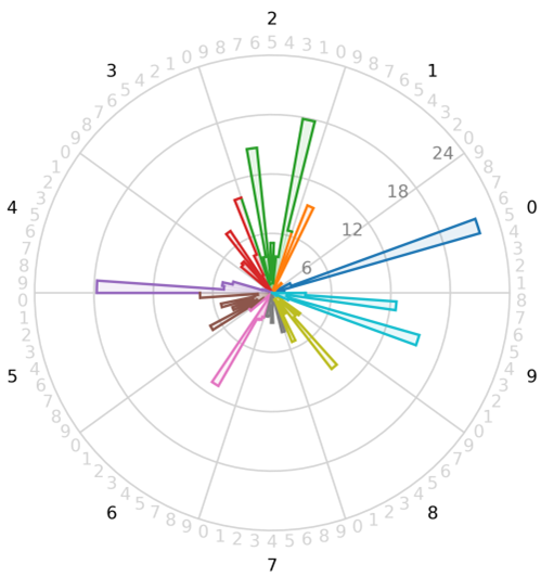 Figure 2: Confustion star.
When small errors hinder the visualization, it is possible to employ the logarithm of the error matrix, see Figure 3. Here, the center of the circle does not correspond to a null error but to an arbitrarily chosen small value (0.01 in the graphic).
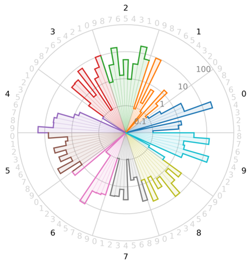 Figure 3: Logarithmic confusion star.
Confusion star for understanding the learning process
Comparing confusion stars at different number of training data can be useful to understand the learning process in addition to the learning curve, see Figure 4.
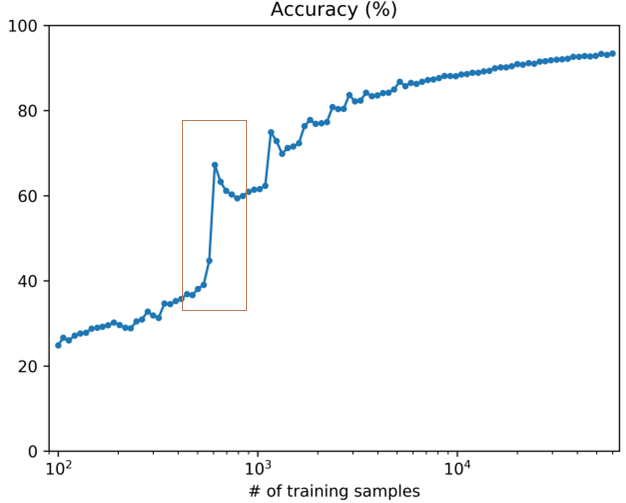 Figure 4: Learning curve of the MNIST dataset using a neural network with a single 128-neurons hidden layer.
Consider the significant increasing in the accuracy occurring around 500 training instances. While the learning curve does not detail what this improvement is due to or how it is distributed in each of the classes, an analysis of the confusion stars can shed more light on the question.
In Figure 5 the confusion stars corresponding to a point with 502 samples (before the jump, accuracy of 38%) and another point with 610 samples (after the jump, accuracy of 67%) are shown. Quite important improvements (smaller errors) can be observed in, for example, the 0 classified as a 2, the 2 classified as a 1, and so on. In other words, the representation of the confusion matrix not only informs us of the overall improvement of the classifier, but also of how this improvement is distributed.
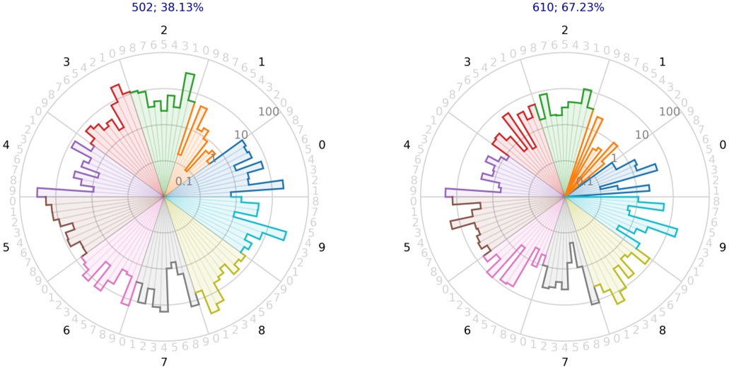 Figure 5: Confusion stars (in logarithmic scale) corresponding to a pair of points before and after the first jump in the learning curve: 502 instances (left; accuracy of 38.13%) and 610 instances (right; accuracy of 67.23%).
Confusion gear plot
The confusion gear plot depicts the non-diagonal elements of the hits matrix \(\mathbf{HM}\) or \(\boldsymbol{\Psi}\) in a circle. So, we have a visual inspection of the classification hits from one class relative to all other ones. Like the confusion star, the circle is divided in \(C\) arcs (one for each class), and each arc is again divided in \(C-1\) sectors (all but the sector corresponding to the relative arc’s class).
Figure 6 depicts the confusion gear for the MNIST example. Consider again class 2 as reference. Here, we se lower values corresponding to class 1 and class 7, according to the higher errors found in Figure 2 or Figure 3. We remark that a perfect classification will results in a full confusion gear.
Since the hits are usually not so small, there is no need to consider logarithm transformations as in confusion stars.
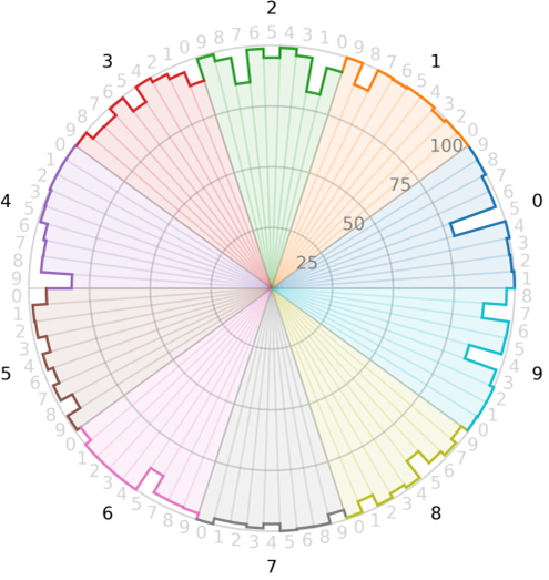 Figure 6: Confusion gear.
Conclusions
A new way of representing the information conveyed by confusion matrices is proposed in the form of a confusion star (focusing on the errors) or a confusion gear (centered on the hits). The new tools successfully represents multiclass classification results in the form of a radial plot.
The traditional way to represent confusion matrix uses colors (and eventually texts) to indicate the number of instances belonging to an actual class that are classified to an estimated class. Instead, confusion stars and gears use shapes to convey that information. Changing colors by shapes significantly improves the readability of the proposed graphics.
An additional property of the confusion stars and gears is that the enclosed area provides information about the overall classification performance. The relation of these areas to standard classification metrics has also been derived.
Finally, the new graphic tools can usefully be employed to visualize the performance of a sequence of classifiers.
References
[1] A. Luque, M. Mazzoleni, A. Carrasco and A. Ferramosca, “Visualizing Classification Results: Confusion Star and Confusion Gear,” in IEEE Access, vol. 10, pp. 1659-1677, 2022, doi: 10.1109/ACCESS.2021.3137630.
[2] L. Deng, “The MNIST Database of Handwritten Digit Images for Machine Learning Research [Best of the Web],” in IEEE Signal Processing Magazine, vol. 29, no. 6, pp. 141-142, Nov. 2012, doi: 10.1109/MSP.2012.2211477.